library(ameras)
#> Loading required package: nimble
#> nimble version 1.4.2 is loaded.
#> For more information on NIMBLE and a User Manual,
#> please visit https://R-nimble.org.
#>
#> Attaching package: 'nimble'
#> The following object is masked from 'package:stats':
#>
#>     simulate
#> The following object is masked from 'package:base':
#>
#>     declare
library(ggplot2)
data(data, package="ameras")
Introduction
For non-Gaussian families, three relative risk models for the main exposure are supported, the usual exponential model RR_i=\exp(\beta_1 D_i+\beta_2 D_i^2+ \mathbf{M}_i^T \mathbf{\beta}_{m1}D_i + \mathbf{M}_i^T \mathbf{\beta}_{m2} D_i^2), the linear(-quadratic) excess relative risk (ERR) model RR_i= 1+\beta_1 D_i+\beta_2 D_i^2 + \mathbf{M}_i^T \mathbf{\beta_{m1}}D_i + \mathbf{M}_i^T \mathbf{\beta}_{m2}D_i^2, and the linear-exponential model RR_i= 1+(\beta_1 + \mathbf{M}_i^T \mathbf{\beta}_{m1}) D_i \exp\{(\beta_2+ \mathbf{M}_i^T \mathbf{\beta}_{m2})D_i\}. This vignette illustrates fitting the three models using regression calibration for logistic regression, but the same syntax applies to all other settings.
Exponential relative risk
The usual exponential relative risk model is given by RR_i=\exp(\beta_1 D_i+\beta_2 D_i^2+ \mathbf{M}_i^T
\mathbf{\beta}_{m1}D_i + \mathbf{M}_i^T \mathbf{\beta}_{m2}
D_i^2), where the quadratic and effect modification terms are
optional (not fit by setting deg=1 and not supplying
modifier, respectively). This model is fit by setting
model="EXP" as follows:
fit.ameras.exp <- ameras(Y.binomial~dose(V1:V10, deg=2, model="EXP")+X1+X2,
                         data=data, family="binomial", methods="RC")
#> Fitting RC
summary(fit.ameras.exp)
#> Call:
#> ameras(formula = Y.binomial ~ dose(V1:V10, deg = 2, model = "EXP") +
#>     X1 + X2, data = data, family = "binomial", methods = "RC")
#>
#> Rows:
#>   Supplied: 3000
#>   Omitted by na.action: 0
#>   Used for fitting: 3000
#>
#> Total CPU runtime: 0.4 seconds
#>
#> CPU runtime in seconds by method:
#>
#>  Method   Fit  CI Total
#>      RC 0.368 0.0 0.368
#>
#> Summary of coefficients by method:
#>
#>  Method         Term Estimate      SE
#>      RC  (Intercept) -0.94461 0.08409
#>      RC           X1  0.44552 0.07667
#>      RC           X2 -0.33376 0.09601
#>      RC         dose  0.37904 0.10388
#>      RC dose_squared  0.01943 0.02750
#>
#> Note: confidence intervals not yet computed. Use confint() to add them.
Linear excess relative risk
The linear excess relative risk model is given by RR_i=1+\beta_1 D_i+\beta_2 D_i^2+ \mathbf{M}_i^T
\mathbf{\beta}_{m1}D_i + \mathbf{M}_i^T \mathbf{\beta}_{m2}
D_i^2, where again the quadratic and effect modification terms
are optional. The degree is specified with deg, as in the
exponential model; the example below uses deg=2. This model
is fit by setting model="ERR" as follows:
fit.ameras.err <- ameras(Y.binomial~dose(V1:V10, deg=2, model="ERR")+X1+X2,
                         data=data, family="binomial", methods="RC")
#> Fitting RC
summary(fit.ameras.err)
#> Call:
#> ameras(formula = Y.binomial ~ dose(V1:V10, deg = 2, model = "ERR") +
#>     X1 + X2, data = data, family = "binomial", methods = "RC")
#>
#> Rows:
#>   Supplied: 3000
#>   Omitted by na.action: 0
#>   Used for fitting: 3000
#>
#> Total CPU runtime: 0.4 seconds
#>
#> CPU runtime in seconds by method:
#>
#>  Method   Fit  CI Total
#>      RC 0.399 0.0 0.399
#>
#> Summary of coefficients by method:
#>
#>  Method         Term Estimate      SE
#>      RC  (Intercept) -0.87359 0.09759
#>      RC           X1  0.44587 0.07672
#>      RC           X2 -0.33552 0.09610
#>      RC         dose  0.04878 0.21283
#>      RC dose_squared  0.28763 0.08100
#>
#> Note: confidence intervals not yet computed. Use confint() to add them.
Linear-exponential relative risk
The linear-exponential relative risk model is given by RR_i= 1+(\beta_1 + \mathbf{M}_i^T
\mathbf{\beta}_{m1}) D_i \exp\{(\beta_2+ \mathbf{M}_i^T
\mathbf{\beta}_{m2})D_i\}, where the effect modification terms
are optional. This model is fit by setting model="LINEXP"
as follows:
fit.ameras.linexp <- ameras(Y.binomial~dose(V1:V10, model="LINEXP")+X1+X2,
                         data=data, family="binomial", methods="RC")
#> Fitting RC
summary(fit.ameras.linexp)
#> Call:
#> ameras(formula = Y.binomial ~ dose(V1:V10, model = "LINEXP") +
#>     X1 + X2, data = data, family = "binomial", methods = "RC")
#>
#> Rows:
#>   Supplied: 3000
#>   Omitted by na.action: 0
#>   Used for fitting: 3000
#>
#> Total CPU runtime: 0.6 seconds
#>
#> CPU runtime in seconds by method:
#>
#>  Method   Fit  CI Total
#>      RC 0.601 0.0 0.601
#>
#> Summary of coefficients by method:
#>
#>  Method             Term Estimate      SE
#>      RC      (Intercept)  -0.9326 0.08592
#>      RC               X1   0.4456 0.07668
#>      RC               X2  -0.3343 0.09603
#>      RC      dose_linear   0.3255 0.11919
#>      RC dose_exponential   0.3455 0.10814
#>
#> Note: confidence intervals not yet computed. Use confint() to add them.
Comparison between models
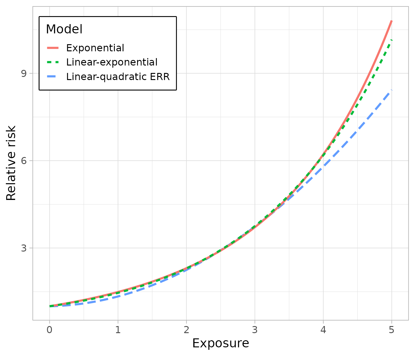
To compare between models, it is easiest to do so visually:
ggplot(data.frame(x=c(0, 5)), aes(x))+
  theme_light(base_size=15)+
  xlab("Exposure")+
  ylab("Relative risk")+
  labs(col="Model", lty="Model") +
  theme(legend.position = "inside",
        legend.position.inside = c(.2,.85),
        legend.box.background = element_rect(color = "black", fill = "white", linewidth = 1))+
  stat_function(aes(col="Linear-quadratic ERR", lty="Linear-quadratic ERR" ),fun=function(x){
    1+fit.ameras.err$RC$coefficients["dose"]*x + fit.ameras.err$RC$coefficients["dose_squared"]*x^2
  }, linewidth=1.2) +
  stat_function(aes(col="Exponential", lty="Exponential"),fun=function(x){
    exp(fit.ameras.exp$RC$coefficients["dose"]*x + fit.ameras.exp$RC$coefficients["dose_squared"]*x^2)
  }, linewidth=1.2) +
  stat_function(aes(col="Linear-exponential", lty="Linear-exponential"),fun=function(x){
    1+fit.ameras.linexp$RC$coefficients["dose_linear"]*x * exp(fit.ameras.linexp$RC$coefficients["dose_exponential"]*x)
  }, linewidth=1.2)